- Categorical data is where the number of observations in different groupings are counted.
- The chi-square test is usually chosen to analyse this type of data. But just because it’s popular doesn’t necessarily mean it’s correct or the best approach.
- Professor Peter Cahusac (Department of Pharmacology & Biostatistics, at the College of Medicine, Alfaisal University, Saudi Arabia) explains why the chi-square test is most often not the best test to choose.
- Instead, he recommends the evidential likelihood approach, a coherent method that avoids the issues caused by significance testing.
Categorical data consists of frequencies of observations that fall into two or more categories. The categories can be organised in one dimension, eg, the number of votes attracted by each of four political parties, to form a one-way table. If we add a second dimension, such as gender, then we have a contingency table showing how men and women vote.
The chi-square test is used to compare observed frequencies with expected frequencies according to a specific hypothesis. The one-way table can be tested for goodness of fit, while the contingency table can be tested for association (or independence) of two variables.

While more than 100 different statistical tests have been devised for all types of data, only around 30 of them regularly appear in research publications. The chi-square test is the most popular test for categorical data and appears in thousands of publications annually across all scientific disciplines. Professor Peter Cahusac at the Department of Pharmacology and Biostatistics, College of Medicine, Alfaisal University, Saudi Arabia, explains why the chi-square test is most often not the best test to use.
Most popular isn’t always best
We all know that being popular doesn’t always mean being correct, or even the best. We will examine the mathematical assumptions needed for the test, and some of the history about statistical inference. But first, let’s look at a couple of examples.
Example 1: Does the addition of suet improve the taste of mince pies?
Twenty-five participants were involved in a study to determine whether adding suet to the mincemeat in mince pies affected taste. Only 5 received pies made with suet and 20 received pies without suet. The contingency table, showing how many participants thought their pie tasted good or not, is given below:

To interpret the data correctly, we need to know whether the proportions of those saying the pies tasted good versus not good was different across the two groups of participants. The proportion of participants saying that suet pies were good was 0.8 (4/5), compared with 0.3 (6/20) for non-suet pies. But we should also consider the proportions in the columns: 0.4 (4/10) of the participants that said the pies that tasted good had suet, versus only 0.067 (1/15) of the participants who said the pies that did not taste good had suet.
The null hypothesis typically states that there is no difference. So, if there was no difference in the row-wise and column-wise proportions, we would say that there is no association between the suet and taste variables, ie, adding suet doesn’t affect the pies’ taste.
The total number of pies that did and didn’t taste good (10 & 15) and the number of pies made with and without suet (5 & 20) are known as the marginal totals. To help us test for any association we need to know, given the marginal totals, what we would expect each of the 4 cells to be if those proportions were identical.
In the following table, we calculate the expected cell values for all 4 cells using the multiplication rule for the probability of the joint occurrence of 2 independent events. The top left entry gives a probability of:

and we multiply this by the total number of people tasting the pies: 0.08×25=2.

For convenience and simplicity in this example, all the expected values are integers. We can carry out a number of different analyses of these data. Here are the results for some of them:
1 Chi-square analysis: X² (1)=4.167, p0.041
2 Chi-square analysis with continuity correction:
X²(1)=2.344, p0.126
3 Fisher’s exact test: p0.121
4 Likelihood ratio test (LRT): G(1)=4.212, p0.040
5 Log likelihood ratio test: S=2.1
6 Log likelihood ratio test for variance: Svar=0.9
So what can we conclude?
The first analysis uses the general formula for chi-square:

The table has r rows and c columns, where we denote the observed count in the ith row and jth column as Oij and the expected value in the ith row and jth column as Eij.

There are restrictions on this analysis. Some say that all expected values should be at least 5, while others claim that up to 20% of expected values can be less than 5. In our example, half of the cells have expected values less than 5, disqualifying this particular analysis.
Some influential statistical textbook authors made great efforts to persuade readers to use likelihood ratio tests.
This means that analyses 1 and 2 listed above should not be done or reported. This now leaves us with tests 3, 4, 5, and 6.
Chi-square test assumptions
The chi-square test is based upon the assumption that the calculated X² values follow an approximation to the χ² distribution. The χ² distribution is theoretical. Mathematically, it produces a continuous range of numbers. For individual cells in a table, it is assumed that their values follow a normal distribution because χ² is the sum of squared normal deviates ∑z² , where each cell provides a z value.

These assumptions are only reasonable when the numbers in most of the cells are sufficiently large. Having small numbers in the cells leads to a couple of related problems. First, there will only be a limited number of possible contingency tables that can be drawn up with those counts. This means that only a limited number of X² values can be calculated, breaking up the continuous nature of the χ² distribution. Secondly, the distribution of values is so limited that it cannot follow the normal distribution required for the summation of the z² values across the table.
The most appropriate test for categorical data, when we are interested in the fit of proportions, is the likelihood ratio test.
However, even if the analysis meets the requirements mentioned above, probably the shortest paper in statistics, published by Ken Williams in 1976, gives a further, rather technical and mathematical, reason why X² should not even be calculated. It reveals that if the difference between the observed and expected frequencies is equal to the expected frequency, in any cell within the table, this would violate the logarithmic expansion of the Mercator series (en.wikipedia.org/wiki/Mercator_series). In contingency tables, this happens when the observed frequency for any cell is 0. Williams concludes saying: ‘As it is now computationally easy to calculate XML[likelihood ratio test] there seems to be no reason for the continued use of Pearson’s approximation [the chi-square test], especially as it is frequently not valid to do so anyway.’
Nothing has changed in almost 50 years since that was written. Students continue to be taught the chi-square test for categorical data, and researchers continue to give X² and associated p values for their data. Some influential statistical textbook authors made great efforts to persuade readers to use likelihood ratio tests. While some of the early reluctance may have been due to the then difficulty in calculating logarithms, nowadays all scientific calculators have a logarithm button, and spreadsheet functions include logarithms.
Example 2: Do 312 randomly selected cards have the expected red and black proportions for court and pip cards?
To increase their house edge, casinos often use multiple decks of cards for blackjack. Let us say that we selected the 312 cards at random from a population of millions of cards produced by the card factory. We might be surprised if we got the following results:

When we do our 6 analyses we get:
1 Chi-square analysis: X²(1)=0.004, p=0.951
2 Chi-square analysis with continuity correction: X² (1)=0.000, p1
3 Fisher’s exact test: p1
4 Likelihood ratio test (LRT): G(1)=0.004, p0.951
5 Log likelihood ratio test for proportions: S=0.002
6 Log likelihood ratio test for variance: Svar=2.3
Even though there is a 3:10 ratio of court to pip cards in the population, would we really expect exactly 72 court cards and 240 pip cards in our randomly selected sample? Also, exactly 36 black and 36 red court cards, really? Probably not, we would rightly be suspicious that the cards were not randomly selected.
With sampling variability we would expect something like this:

The first table looks ‘too good to be true’. How do we measure our surprise or suspicion that the cards were not randomly selected?
Likelihood
Likelihood was first defined by Sir Ronald Fisher more than 100 years ago. It is a distinct concept from probability though it is proportional to it. He suggested that hypotheses could be compared using likelihood ratios. Later in his life Fisher endorsed the likelihood ratio approach:
‘For all purposes, and more particularly for the communication of the relevant evidence supplied by a body of data, the values of the Mathematical Likelihood are better fitted to analyse, summarize, and communicate statistical evidence…’
He suggested that the log likelihood ratio is particularly convenient because independent sources of statistical evidence can literally be added together.
For a table of categorical data, using the same symbols as previously (equation 1) we would use this to calculate the log likelihood (LL) for the observed values given the same observed values:

Should any observed frequency be zero, then by convention the term 0×ln(0) = 0. The log likelihood for the expected values given the observed values would be:

Their ratio which gives us the log likelihood ratio:

In his classic book titled Likelihood, Anthony Edwards FRS promoted the likelihood approach and made considerable efforts to clarify the use of the chi-square test, stating that the chi-square test is assessing the variance of the frequencies, rather than their fit to proportions specified by a hypothesis. We are usually interested in how the frequencies fit a particular hypothesis, rather than their variance in the table, and he argued that the log likelihood ratio was optimal for this purpose.
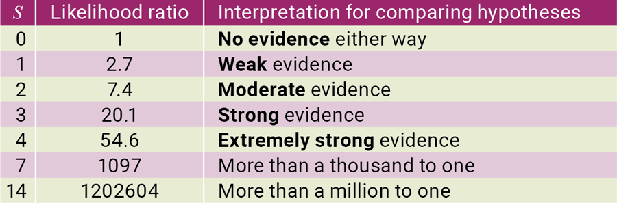
It all depends on the question you are trying to answer. In example 1, we were interested in whether the data suggested that there was an association between suet and how good the pies tasted. The proportions did not support the hypothesis that the two variables were independent, and therefore that hypothesis was rejected. We obtained S=2.1, which means moderate evidence (see Table 5) that there is an association between whether or not suet was used in the pies and their appreciation. In example 2, we are suspicious that the data fit the hypothesis too well, that is, their variance is smaller than expected.
To interpret S we should refer to this table:
Data that is too good to be true
Edwards derived a formula that gives an S value for the variance of the frequencies. This was adapted for the more general case where df is the degrees of freedom for the table:

The X² is calculated in the usual way using equation 1. For our example 2 data we obtain Svar=2.3. Referring to Table 1 tells us that we should be moderately suspicious of foul play.
Take-home messages
Different tests can be used on the data, depending on the question we want to answer. The most appropriate test for categorical data, when we are interested in the fit of proportions, is the LRT. This approach avoids violating assumptions, and avoids using any corrections. Even better is the S value which is an objective measure of evidence between competing hypotheses. Unlike p value calculations, S is not affected by transformations of variables. Additional data can be added and independently collected data – eg, in a meta-analysis – can be summed.In categorical analyses, S values are additive, which is especially useful for sub-tables of a large contingency table and in multidimensional contingency tables.
While the chi-square test should very rarely be used for categorical data, it can be used when we think that the data is too good to be true, ie, where the variance of the data is suspect. An alternative is to use Svar which incorporates X² in its formula and doesn’t require the use of p values.

Finally, Professor Cahusac’s jamovi module, jeva, can be used for log likelihood analyses (see blog.jamovi.org/2023/02/22/jeva.html). There is a great introduction to the likelihood approach provided by Dr Mircea Zloteanu from Kingston University London: mzloteanu.substack.com/p/a-secret-third-way-likelihoodist.